Page 140 - The Ontario Curriculum, Grades 11 and 12: Mathematics, 2007

Grade 12, College Preparation
2. Modelling Graphically
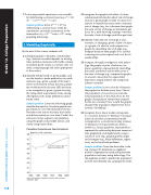
Canadian Greenhouse Gas Emissions
0.8 Gigatons of CO2
0.7 0.6 0.5 0.4 0.3 0.2 0.1
0.0
1980 1984
equivalent
Kyoto benchmark 􏰀
1988 1992
1996 2000
Source: Environment Canada, Greenhouse Gas Inventory 1990-2001, 2003
THE ONTARIO CURRICULUM, GRADES 11 AND 12 | Mathematics
138
1.7 solve exponential equations in one variable by determining a common base (e.g., 2x = 32, 45x − 1 = 22(x + 11), 35x + 8 = 27x)
Sample problem: Solve 35x + 8 = 27x by determining a common base, verify by substitution, and make connections to the intersection of y = 35x + 8 and y = 27x using graphing technology.
By the end of this course, students will:
2.1 interpret graphs to describe a relationship (e.g., distance travelled depends on driving time, pollution increases with traffic volume, maximum profit occurs at a certain sales vol- ume), using language and units appropriate to the context
2.2 describe trends based on given graphs, and use the trends to make predictions or justify decisions (e.g., given a graph of the men’s 100-m world record versus the year, predict the world record in the year 2050 and state your assumptions; given a graph showing the rising trend in graduation rates among Aboriginal youth, make predictions about future rates)
Sample problem: Given the following graph, describe the trend in Canadian greenhouse gas emissions over the time period shown. Describe some factors that may have influ- enced these emissions over time. Predict the emissions today, explain your prediction using the graph and possible factors, and verify using current data.
2.3 recognize that graphs and tables of values communicate information about rate of change, and use a given graph or table of values for a relation to identify the units used to measure rate of change (e.g., for a distance–time graph, the units of rate of change are kilometres per hour; for a table showing earnings over time, the units of rate of change are dollars per hour)
2.4 identify when the rate of change is zero, constant, or changing, given a table of values or a graph of a relation, and compare two graphs by describing rate of change (e.g., compare distance–time graphs for a car that is moving at constant speed and a car that is accelerating)
2.5 compare, through investigation with techno- logy, the graphs of pairs of relations (i.e., linear, quadratic, exponential) by describing the initial conditions and the behaviour of the rates of change (e.g., compare the graphs of amount versus time for equal initial deposits in simple interest and compound interest accounts)
Sample problem: In two colonies of bacteria, the population doubles every hour. The ini- tial population of one colony is twice the initial population of the other. How do the graphs of population versus time compare for the two colonies? How would the graphs change if the population tripled every hour, instead of doubling?
2.6 recognize that a linear model corresponds
to a constant increase or decrease over equal intervals and that an exponential model corresponds to a constant percentage increase or decrease over equal intervals, select a model (i.e., linear, quadratic, exponential) to represent the relationship between numerical data graphically and algebraically, using a variety of tools (e.g., graphing technology) and strategies (e.g., finite differences, regres- sion), and solve related problems
Sample problem: Given the data table at the top of page 139, determine an algebraic model to represent the relationship between population and time, using technology. Use the algebraic model to predict the population in 2015, and describe any assumptions made.